The Birthday Problem

What is it?

The Birthday Problem describes the probability of a pair of individuals sharing the same birthday, in a sample of n individuals. In our group of 75 students in med school, 2 or 3 pairs of us shared the exact same birthday (day and month). This seemed to be an unexpectedly high frequency, considering that the probability of a person’s birthday being a particular day of the year is 1/365. But in fact, as the Wikipedia article explains, this is not all that surprising. In a group of 75, it turns out, there is near certainty that a pair of individuals would share the same birthday. But in this calculation, it is assumed that it is equally probable for a person to be born on any day of the year.

I thought I’d use some real life data to empirically test this (while also practising data analysis in R). I found that it is not very easy to obtain a large dataset with birth dates for the UK. I eventually came across the National Bureau of Economic Research which had US vitality statistics for the years 1968 - 2013. But even here, I learnt that full birth dates (dd-mm-yy) are only available till 1988.

I first downloaded the 1988 and 2013 datasets and plotted the total number of births (normalized by number of days in each month).

library(data.table)
library(ggplot2)
# download and unzip http://www.nber.org/data/vital-statistics-natality-data.html  
 # 2013  
#download.file(url = "http://www.nber.org/natality/2013/natl2013.csv.zip", destfile = "./R programming assignments/births/natl2013.csv.zip")  
#unzip(zipfile = "./R programming assignments/births/natl2013.csv.zip", exdir = "./R programming assignments/births")  
#births2013 <- fread(input = "./R programming assignments/births/natl2013.csv", select = "dob_mm") # ~ 2.5 GB file  
# 1988  
#download.file(url = "http://www.nber.org/natality/1988/natl1988.csv.zip", destfile = "./R programming assignments/births/natl1988.csv.zip")  
#unzip(zipfile = "./R programming assignments/births/natl1988.csv.zip", exdir = "./R programming assignments/births")  
#births1988 <- fread(input = "./R programming assignments/births/natl1988.csv", select = c("birmon", "birday")) # ~ 1.26 GB
#save(births2013, births1988, file = "datasets.Rdata")
load("datasets.Rdata") 
# generate useful vectors  
 daysinmonth <- c(31, 28, 31, 30, 31, 30, 31, 31, 30, 31, 30, 31)  
 daysinmonthleap <- c(31, 29, 31, 30, 31, 30, 31, 31, 30, 31, 30, 31)
  
 # explore  
 birthsbymonth2013 <- table(births2013$dob_mm) # births by month  
 plot(birthsbymonth2013/daysinmonth, ylim = c(0,12000), type = "l") # normalised to no. of days in each month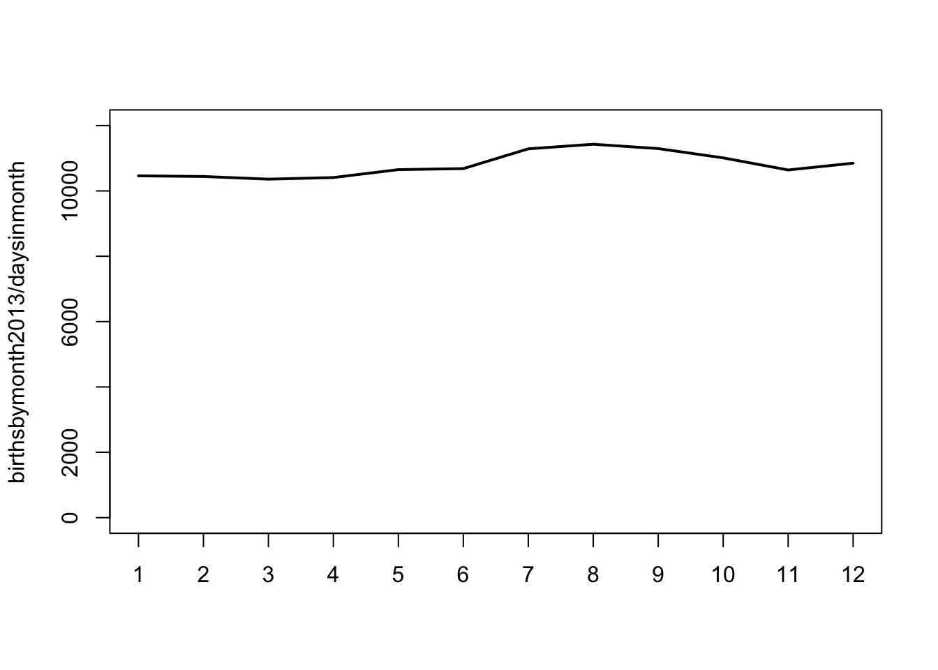  

 birthsbymonth1988 <- table(births1988$birmon) # births by month  
 plot(birthsbymonth1988, type = "l") # raw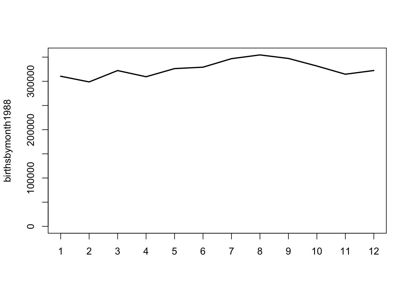  

 plot(birthsbymonth1988/daysinmonthleap, ylim = c(0,12000), type = "l") # normalised to no. of days in each month (leap year)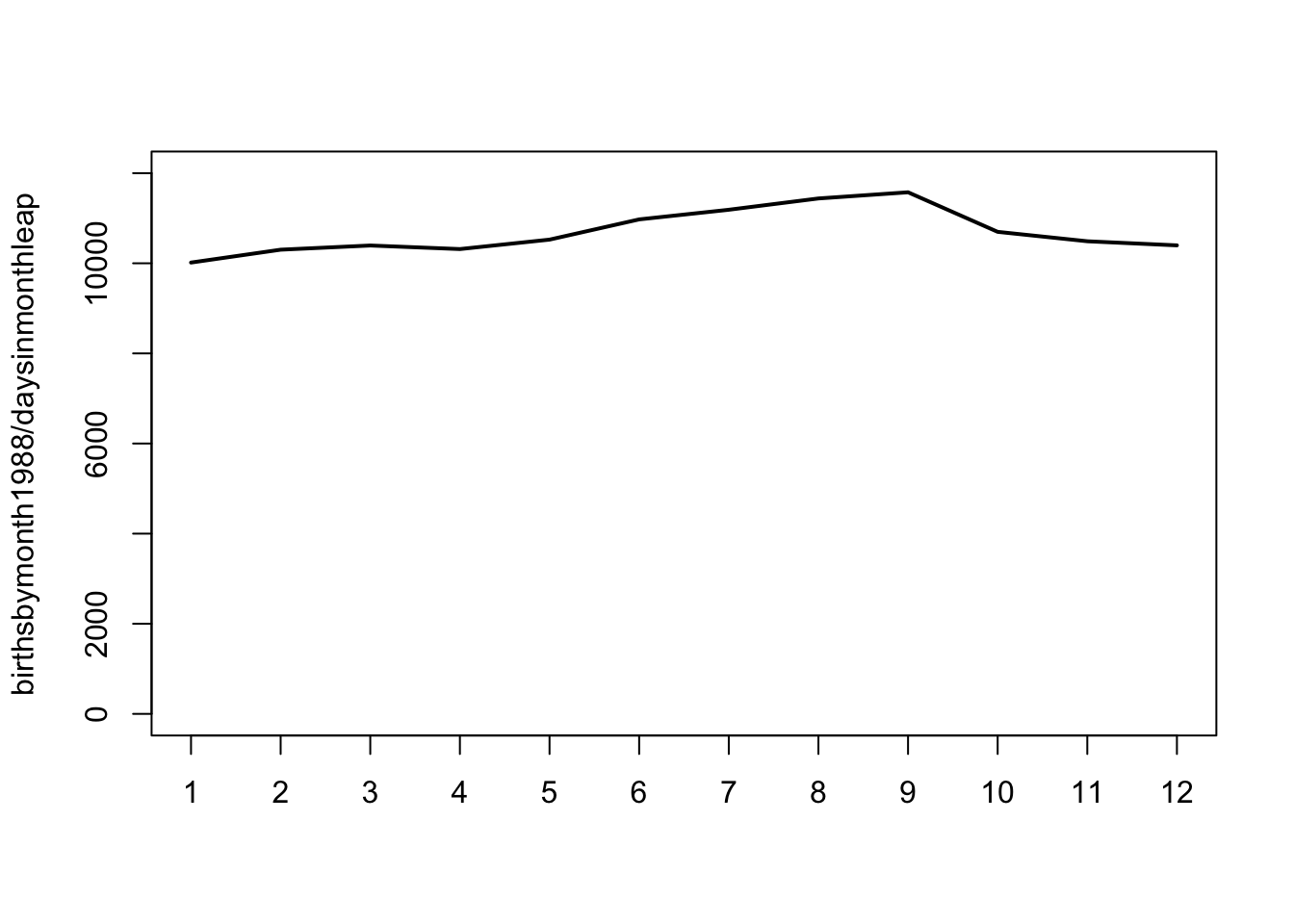  

 # add columns to data  
 births1988[,ddmm:=paste(birday, birmon, sep = "-")] # new column with day and month combined  
 # The Birthday Problem  
 rowsin1988 <- nrow(births1988) # store number of rows to avoid calculating in each iteration of for loop  
 bdayproblem <- data.table("samplesize" = integer(0), "duplicates" = integer(0)) # empty data atable  

Did you notice that the 2013 dataset is 2.5 GB? And the fread() function in R takes a mere 40 seconds to load all of it! You’ll notice that I loaded only the month and day columns for the 1988 dataset to avoid using up too much memory.

There seems to be higher number of births between months 6 to 9 in both 1988 and 2013, although this is only ~20% increase at its peak compared to, say, January. (Interestingly, there is a skewed distribution of birthdays in our lab too, with a high distribution in the months of July and August). How does this skewed distribution affect the probability of a pair having the same birthday in a group of g randomly picked individuals?

R has a handy function to pick n random numbers between x to y. The following function picks a given number of random rows in the entire 1988 dataset, selects the date (dd-mm) in those particular rows, and determines if there is at least one pair of duplicate dates (i.e., whether 2 individuals share the same birthday. The function then returns the sample size and a boolean value (1 = at least one duplicate found, 0 = no duplicates found in the given sample).

 # function returns list of samplesize and boolean of presence of 1 or more duplicates (0 = no duplicates, 1 = at least 1 duplicate)  
 calcduplicates <- function(data = births1988, samplesize = 70, numberofrows = rowsin1988){  
  return(list(samplesize, as.numeric(sum(duplicated(data[sample(numberofrows, samplesize), 3, with = FALSE])) > 0)))  
 }  

Now, it’s just a matter of looping this many many times (I did it a 100 times; the larger this number, the smoother the curve, obviously.) to obtain a probability. And wrap that in another loop for sample sizes from 2 to 100.

 # for loop  
 for (g in 2:100) { # in a group of g people  
  for (n in 1:100) { # perform random sampling n times  
   bdayproblem <- rbind(bdayproblem, calcduplicates(samplesize = g))  
  }  
 }  

And finally, I reduced the individual observations to fractions (number of times duplicates were found per 1000 iterations) and plotted them, along with geom_smooth() to add a regression line.

 # summarise data  
 samplesizevsprobability <- tapply(X = bdayproblem$duplicates, INDEX = bdayproblem$samplesize, mean) # calculate mean of the "duplicates" column  
 samplesizevsprobability <- data.table(samplesize = as.numeric(names(samplesizevsprobability)), probability = samplesizevsprobability) # convert to dataframe  
 # plot  
 #png(filename = "./R programming assignments/births/alldata_probability.png", width = 1550, height = 1000)  
 ggplot(data = samplesizevsprobability, aes(x = samplesize, y = probability)) + geom_line(color = "darkblue", size = 2) + geom_smooth(color = "black") + geom_vline(aes(xintercept = 23), linetype = 2) + theme(axis.text = element_text(size=20), axis.title = element_text(size=20, face = "bold"))# plot data  

## Warning: Using `size` aesthetic for lines was deprecated in ggplot2 3.4.0.
## ℹ Please use `linewidth` instead.
## This warning is displayed once every 8 hours.
## Call `lifecycle::last_lifecycle_warnings()` to see where this warning was
## generated.

## `geom_smooth()` using method = 'loess' and formula = 'y ~ x'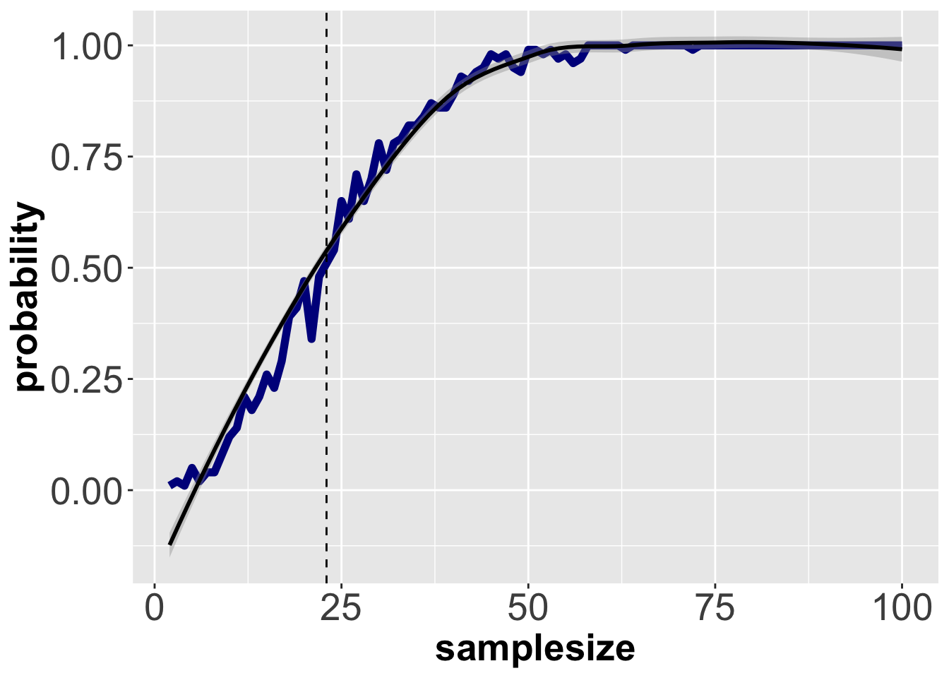

 #dev.off()  

The dotted line (x = 23) intersects the curve at y = ~0.5, which is close to the predicted value. So the slight skew in real-life birth data does not seem to have much effect on the probability curve. It would be interesting to see how much of a skew required to see a noticeable effect on the curve (if at all?). And what about leap days?

Going back to the sample size of 75 from my med school, it turns out the number of birthday pairs is in fact lower than expected, as running the above function with 1000 iterations (with sample size = 75) gives a mean duplicate number of ~7.

 dupfor75 <- numeric()  
 for (i in 1:100) {dupfor75 <- c(dupfor75, sum(duplicated(births1988[sample(rowsin1988, 75), 3, with = FALSE])))}  
 mean(dupfor75) 

## [1] 7.12

Any suggestions on how to do the same analysis faster, or on how to improve it, are of course welcome.

Further reading

1. Decline and loss of birth seasonality in Spain: analysis of 33 421 731 births over 60 years